Using the watershed algorithm for Cell Based Segmentation from blood smears (part 1)

Since when did a super interesting blog become a bio lesson?

Sometimes you get inspired by the things you’re most horrible at. In my final year of school, I decided to face one of my biggest science-field nightmares, biology. However, if I’m doing bio, it’s on my terms. No memorizing for an exam or profusely exhibiting my medical adroitness through unnecessarily labyrinthine jargon. Also, I’m competing in a competition where I’m creating a neural network to detect pathogens in blood smears.

Introduction to blood smears

To put it concisely, a blood smear is essentially a microscopic image of your blood that contains a set of Red blood cells, white blood cells and other blood cell nonsense. It looks similar to this

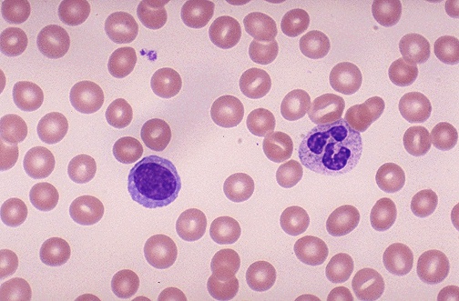
These can reveal a lot about your present health. Blood morphology (viewing and understanding the composition of blood smear images) can point to the onset of leukemia, sickle cell, and also the presence of lymphocytes, monocytes, basophil’s etc. It generally requires a trained eye to detect all of  this, but during the next few lessons, we’re going to see if we can make a computer segment the blood cells and understand them individually.

Prerequisites

A very solid foundation in OpenCV and Python; this exercise is just another big project you’ll be undertaking to hone your skills so you should ideally have a good understanding of the basic functions or if not, have the ability to look up and process the documentation.

Watershed? Why not contours?

For the sake of simplicity and to avoid too many gifs and animations, I’m just going to say it’s because you can learn an amazing new skill and learn how to implement it. However, if you’d like to see all the gifs and animations, check this brilliant page out. It’s where I learnt about watershed.

Morphology

In order to apply watershed, you’ll need to use morphological transformations and contrast enhancement in order to define boundaries and markers for the algorithm to take effect properly. Not doing these may lead to over-segmentation or under-segmentation.

#load your image, I called mine 'rbc'
img = cv2.imread('C:\Users\\user pc\Desktop\PPictures\\rbc.jpg')
#keep resizing your image so it appropriately identifies the RBC's
img = cv2.resize (img, (0,0), fx=5, fy=5)
#it's always easier if the image is copied for long pieces of code.
#we're copying it twice for reasons you'll see soon enough.
wol = img.copy()
gg=img.copy()
#convert to grayscale
img_gray = cv2.cvtColor(gg, cv2.COLOR_BGR2GRAY)
#enhance contrast (helps makes boundaries clearer)
clache = cv2.createCLAHE(clipLimit=2.0, tileGridSize=(8,8))
img_gray = clache.apply(img_gray)
#threshold the image and apply morphological transforms
_, img_bin = cv2.threshold(img_gray, 50, 255,
        cv2.THRESH_OTSU)
img_bin = cv2.morphologyEx(img_bin, cv2.MORPH_OPEN,
        numpy.ones((3, 3), dtype=int))
img_bin = cv2.morphologyEx(img_bin, cv2.MORPH_DILATE,
        numpy.ones((3, 3), dtype=int), iterations= 1)
#call the 'segment' function (discussed soon)
dt, result = segment(img, img_bin)

Apply watershed

Prior to applying watershed, a Euclidean distance transform is first implemented onto the frame. This evaluates the brightness of each pixel relative to it’s distance to a pixel with a ‘zero’ value. A zero value pixel is black, so EDT allows for a visualization of the how far any part of the image is from the background (which due to previous thresholding, should be black). You’ll notice that areas around the edge have a duller gray color, that slowly becomes a bright white color. We want to focus on the bright white color as our marker, because we’re sure it’s a part of the shape. The edges and duller colors are not 100%.

def segment(im1, img):
    #morphological transformations
    border = cv2.dilate(img, None, iterations=10)
    border = border - cv2.erode(border, None, iterations=1)
    #invert the image so black becomes white, and vice versa
    img = -img
    #applies distance transform and shows visualization
    dt = cv2.distanceTransform(img, 2, 3)
    dt = ((dt - dt.min()) / (dt.max() - dt.min()) * 255).astype(numpy.uint8)
    #reapply contrast to strengthen boundaries
    clache = cv2.createCLAHE(clipLimit=2.0, tileGridSize=(8,8))
    dt = clache.apply(dt)
    #rethreshold the image
    _, dt = cv2.threshold(dt, 40, 255, cv2.THRESH_BINARY)
    lbl, ncc = label(dt)
    lbl = lbl * (255/ncc)
    # Complete the markers
    lbl[border == 255] = 255

    lbl = lbl.astype(numpy.int32)
    #apply watershed
    cv2.watershed(im1, lbl)

    lbl[lbl == -1] = 0
    lbl = lbl.astype(numpy.uint8)
    #return the image as one list, and the labels as another.
    return dt, lbl

And there you have it! You can Segment most blood smear images in a few seconds! A major problem, however, is its lack of accuracy for different sized images of various resolutions and color textures. In order to improve the accuracy, I’ll soon be showing you how to do the same morphology, except with histogram equalization so you can more clearly define your boundaries.