FIRST and foremost, my blog has a non-chronological arrangement. Instead of posting the most recent posts on top, I have posted them in order of ‘coolness’, a completely non-subjective, reliable scientific unit of measurement. So if you scroll down and see that there’s a 3 month gap between my posts, please understand that this is because I have chosen to include my best work on top, and scrolling down will reveal to you the MULTITUDE of other tutorials.
SECOND and Eyebrowmost (because the Eyebrow is below the fore(head), just as second is below the first. Its fine, don’t thank me for the enlightenment),The lack of tutorials in recent months is because I don’t have full ownership to disclose FIREFLY to the public, as I’m competing in a competition. I promise guys, as soon as we hit the 18th of March, be ready for a barrage of code and tutorials showing you guys how to effectively use ROS to simulate and program autonomous drones.
This project is probably a 110% improvement to my Google Science Fair project. It uses an Artificial Intelligence trained in Python, it can read evacuation maps on its own and capitalizes on the way birds see to create a supreme obstacle avoidance system. FIREFLY is a drone platform for autonomous, low cost rapid evacuation of high-rise buildings.
Thanks to Dennis Shehadeh for creating my UAE Drones for Good Competition video.
Instructions on how to recreate the computer vision portion of this coming soon!
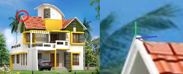
After building a portion of your foundation, it’s best to continue learning by building something that’s not only useful, but also looks insanely impressive. So here you have it, a basic angle calculator.
UPDATE: WordPress is changing some of my code blocks to ‘amp’ and I haven’t yet found a way to fix this. For further guidance (although it would be a good exercise to infer), head over to my github repository.
This tutorial assumes you have some degree of proficiency with Python and can reasonably understand the OpenCV code here.
Determine HSV Range (again)
Before you continue writing the code you’ll need to use this HSV Trackbar to determine the Hue Low/High, Saturation Low/High and Value Low/High for the object you want to track. Mess around with the trackbars until you can only see the color of the object you are looking for. Repeat this process twice, for 2 differently colored objects. Note these values down, you will need them for later.
Filter for HSV Colors
Creating functions makes life a billion times easier, and allows you to organize your code much more effectively. I wrote the code initially with the functions findorange and findblue , although I eventually ended up using green and orange.
#import libs
import cv2
import numpy as np
import math

#uses distance formula to calculate distance
def distance((x1, y1), (x2,y2)):
    dist = math.sqrt((math.fabs(x2-x1))**2+((math.fabs(y2-y1)))**2)
    return dist

#filters for blue color and returns blue color position.
def findblue(frame):
    maxcontour = None
    blue = cv2.cvtColor(frame, cv2.COLOR_BGR2HSV)
    bluelow = np.array([55, 74, 0])#replace with your HSV Values
    bluehi = np.array([74, 227, 255])#replace with your HSV Values
    mask = cv2.inRange(blue, bluelow, bluehi)
    res = cv2.bitwise_and(frame, frame, mask=mask)

#filters for orange color and returns orange color position.
def findorange(frame):
    maxcontour = None
    orange = cv2.cvtColor(frame, cv2.COLOR_BGR2HSV)
    orangelow =  np.array([0, 142, 107])#replace with your HSV Values
    orangehi = np.array([39, 255, 255])#replace with your HSV Values
    mask = cv2.inRange(orange, orangelow, orangehi)
    res = cv2.bitwise_and(frame, frame, mask=mask)
Just remember to change the bluelow and bluehi and orangelow and orangehi array’s elements to those that suit your color choice. All of the functions used should be familiar from my tutorial on ‘Object Tracking and Following with OpenCV Python‘; read that if you don’t get some of it. What we’ve essentially done is sent the initial frame as a parameter to each of these functions, where they then convert to HSV and threshold for the color.
Return object positions
Next, you want to continue building on findblue() and findorange() by allowing them to return the coordinates of your objects.
def findblue(frame):
    blue = cv2.cvtColor(frame, cv2.COLOR_BGR2HSV)
    bluelow = np.array([55, 74, 0])#replace with your HSV Values
    bluehi = np.array([74, 227, 255])#replace with your HSV Values
    mask = cv2.inRange(blue, bluelow, bluehi)
    res = cv2.bitwise_and(frame, frame, mask=mask)
    cnts, hir = cv2.findContours(mask, cv2.RETR_TREE, cv2.CHAIN_APPROX_SIMPLE)
    if len(cnts) >0:
        maxcontour = max(cnts, key = cv2.contourArea)

        #All this stuff about moments and M['m10'] etc.. are just to return center coordinates
        M = cv2.moments(maxcontour)
        if M['m00'] > 0 and cv2.contourArea(maxcontour)>2000:
            cx = int(M['m10'] / M['m00'])
            cy = int(M['m01'] / M['m00'])
            return (cx, cy), True
        else:
            #(700,700), arbitrary random values that will conveniently not be displayed on screen
            return (700,700), False
    else:
        return (700,700), False
#filters for orange color and returns orange color position.
def findorange(frame):
    orange = cv2.cvtColor(frame, cv2.COLOR_BGR2HSV)
    orangelow =  np.array([0, 142, 107])#replace with your HSV Values
    orangehi = np.array([39, 255, 255])#replace with your HSV Values
    mask = cv2.inRange(orange, orangelow, orangehi)
    res = cv2.bitwise_and(frame, frame, mask=mask)
    cnts, hir = cv2.findContours(mask, cv2.RETR_TREE, cv2.CHAIN_APPROX_SIMPLE)
    if len(cnts) >0:
        maxcontour = max(cnts, key = cv2.contourArea)
        M = cv2.moments(maxcontour)
        if M['m00'] > 0 and cv2.contourArea(maxcontour)>2000:
            cx = int(M['m10'] / M['m00'])
            cy = int(M['m01'] / M['m00'])
            return (cx, cy), True
        else:
            return (700,700), False
    else:
        return (700,700), False
The cv2.Moments function and the cx and cy variable declarations are best explained in OpenCV’s introduction to contours. But simply put, lines n – n just return the coordinates of the center of the contour.
The reason we have the blogic boolean variable is just to validate that the object is present on screen. If the object isn’t present, this variable will be set to False, and the coordinates will be (700,700). I chose this set of points arbitrarily, as these, even when plotted, couldn’t be seen on my 300 x 400 window.
Distance Function
We’ll be using trigonometry to calculate the angle, so for this you’ll need to create a function that measures the distance between both points. For this, we use the standard distance equation you should’ve learnt in high school.
#uses distance formula to calculate distance
def distance((x1, y1), (x2,y2)):
    dist = math.sqrt((math.fabs(x2-x1))**2+((math.fabs(y2-y1)))**2)
    return dist
Main Loop
#capture video
cap = cv2.VideoCapture(0)

while(1):
    _, frame = cap.read()
#if you're sending the whole frame as a parameter,easier to debug if you send a copy
    fra = frame.copy()

     #get coordinates of each object
    (bluex, bluey), blogic = findblue(fra)
    (orangex, orangey), ologic = findorange(fra)
    #draw two circles around the objects (you can change the numbers as you like)
    cv2.circle(frame, (bluex, bluey), 20, (255, 0, 0), -1)
    cv2.circle(frame, (orangex, orangey), 20, (0, 128, 255), -1)
Our foundation is set. We’ve made a program that tracks the position of 2 different colored objects on screen, next, we need to apply trig to calculate the angle and display the entire setup in the most grandiose manner possible.
    if blogic and ologic:
        #quantifies the hypotenuse of the triangle
        hypotenuse =  distance((bluex,bluey), (orangex, orangey))
        #quantifies the horizontal of the triangle
        horizontal = distance((bluex, bluey), (orangex, bluey))
        #makes the third-line of the triangle
        thirdline = distance((orangex, orangey), (orangex, bluey))
        #calculates the angle using trigonometry
        angle = np.arcsin((thirdline/hypotenuse))* 180/math.pi

        #draws all 3 lines
        cv2.line(frame, (bluex, bluey), (orangex, orangey), (0, 0, 255), 2)
        cv2.line(frame, (bluex, bluey), (orangex, bluey), (0, 0, 255), 2)
        cv2.line(frame, (orangex,orangey), (orangex, bluey), (0,0,255), 2)
Our code is officially complete…sort of. If you run it, it’ll look great and work great but you’ll notice that it won’t detect any angle over 90 degrees. If you’re familiar with trig, you’ll know why, but to evade this situation and allow it to calculate angles until 180 degrees, we need a few more lines of code.
     #Allows for calculation until 180 degrees instead of 90
if orangey < bluey and orangex > bluex:
    cv2.putText(frame, str(int(angle)), (bluex-30, bluey), cv2.FONT_HERSHEY_SCRIPT_COMPLEX, 1, (0,128,220), 2)
elif orangey < bluey and orangex < bluex:
    cv2.putText(frame, str(int(180 - angle)),(bluex-30, bluey), cv2.FONT_HERSHEY_SCRIPT_COMPLEX, 1, (0,128,220), 2)
elif orangey > bluey and orangex < bluex:
    cv2.putText(frame, str(int(180 + angle)),(bluex-30, bluey), cv2.FONT_HERSHEY_SCRIPT_COMPLEX, 1, (0,128,220), 2)
elif orangey > bluey and orangex > bluex:
    cv2.putText(frame, str(int(360 - angle)),(bluex-30, bluey), cv2.FONT_HERSHEY_SCRIPT_COMPLEX, 1, (0,128, 229), 2)
if k == ord('q'): break
And that’s it! If the object tracker didn’t impress already, now you have a live angle calculator using just your camera.
Object tracking and the concepts learnt from developing an object tracking algorithm are necessary for computer vision implementation in robotics. By the end of this tutorial, you will have learnt to accurately track an object across the screen.
UPDATE: WordPress is changing some of my code blocks to ‘amp’ and I haven’t yet found a way to fix this. For further guidance (although it would be a good exercise to infer), head over to my github repository.
Prerequisites
This tutorial assumes you have some degree of proficiency with Python and can reasonably understand the OpenCV code here.
Determine HSV Range
Before you continue writing the code you’ll need to use this HSV Trackbar to determine the Hue Low/High, Saturation Low/High and Value Low/High for the object you want to track. Mess around with the trackbars until you can only see the color of the object you are looking for. Note these values down, you will need them for later.
Filter for HSV Color
#import necessary libraries
import cv2
import numpy as np
import time
#initialize the video stream
cap = cv2.VideoCapture(0)

#make two arrays, one for the points, and another for the timings
points = []
timer = []
while True:
    #start the timing
    startime = time.time()

    #append the start time to the array named 'timer'
    timer.append(g)

    #you only want to use the start time, so delete any other elements in the array
    del timer[1:]
    _, frame = cap.read()

    #resize and blur the frame (improves performance)
    sized = cv2.resize(frame, (600, 600))
    frame = cv2.GaussianBlur(sized, (7, 7), 0)

    #convert the frame to HSV and mask it
    hsv = cv2.cvtColor(frame, cv2.COLOR_BGR2HSV)
#fill in the values you obtained previously over here
    hlow = 17
    slow = 150
    vlow = 24
    hhigh = 78
    shigh = 255
    vhigh = 255
    HSVLOW  = np.array([hlow, slow, vlow])
    HSVHIGH = np.array([hhigh, shigh, vhigh])
    mask = cv2.inRange(hsv,HSVLOW, HSVHIGH)
    res = cv2.bitwise_and(frame,frame, mask =mask)
All of this stuff should be pretty straightforward after a few read-through’s. The only new function here is cv2.resize() and that itself is quite self explanatory (it resizes the frame). At this point, we have our new, ‘thresholded’ frame.
As a word of advice, make sure there isn’t a huge concentration of the color you’re looking for on the screen. For this basic object tracker, we’re only relying on color so if you have a lot of the color you want to track in the background, your best bet is to find a different colored object.
Find Maximum Contour
A lot of the time, you can simply visualize the algorithm necessary for solving most computer vision problem for robots if you understand what contours are. Since it is such a powerful tool, I suggest you build your foundation at this link (do the exercises, don’t just read), and come back when you kind of understand what contours are.
Once your done, try understanding this code.
    #create an edged frame of the thresholded frame
    edged = cv2.Canny(res, 50, 150)

    #find contours in the edged frame and append to the 'cnts' array
    cnts = cv2.findContours(edged, cv2.RETR_TREE, cv2.CHAIN_APPROX_SIMPLE)[0]

    # if contours are present
    if len(cnts)> 0:

        #find the largest contour according to their enclosed area
        c = max(cnts, key=cv2.contourArea)

        #get the center and radius values of the circle enclosing the contour
        (x, y), radius = cv2.minEnclosingCircle(c)
We started with the cv2.Canny() function (documentation) with a min and max threshold. Ignore the technicalities of the numbers, that essentially finds all of the edges in the frame.
Since cv2.findContours() returns a list, we need to find the largest contour (which we assume is our object) in this list. We use the max(cnts, key=cv2.contourArea). Thus, this function finds the area of all of the contours in the list, and then returns it’s maximum.
Following that we use the cv2.minEnclosingCircle(c) function to find the (x,y) coordinates of the center of the circle, and it’s radius.
At this point, we have tracked our object in the frame. All that’s left is to draw the circle and the trailing line.
        centercircle = (int(x), int(y))
        radius = int(radius)
        cv2.circle(sized, centercircle, radius, (255, 30,255), 2) #this circle is the object
        cv2.circle(sized, centercircle, 5, (0, 0, 255), -1) #this circle is the moving red dot
        points.append(centercircle) #append this dot to the 'points' list
        if points is not None:
            for centers in points:
                cv2.circle(sized, centers, 5, (0, 0, 255), -1) #make a dot for each of the points

    #show all the frames and cleanup
    cv2.imshow('frame', sized)
    cv2.imshow('mask', res)
    k = cv2.waitKey(5) & 0xFF
    g = time.time()
    timer.append(g)

    #if 10 seconds have passed, erase all the points
    delta_t = timer[1] - timer[0]
    if delta_t >= 10:
        del timer[:]
        del points[:]
    if k == 27:
        break
Lines 1-9 essentially draw the circle around the object, and draw another small red circle at it’s center. This dot constitutes a point in the trail. This point is then appended to the existing array ‘points’.
The for loop that follows cycles through each of the centers’ (x,y) coordinates (from the ‘points’ array) and draws another red dot in each position, effectively creating the trail.
Finally, another value is appended to the timer array. Delta_t computes the difference between the start and final times. If this value is greater than 10, all points are erased and a new trail is begun.
Everybody knows how annoying the cv2.imshow() function is, especially when debugging. We need to keep creation names for the first parameter of the function, which tends to interrupt the flow and hang your program if you have a slow computer. Add or import this function to make life easier.
import cv2
import numpy as np
window = 1
def imshow(img):
    global window
    name = "Window %d" %(window)
    window +=1
    cv2.imshow(name, img)
Don’t begin this exercise until you’re familiar with the basic image processing techniques (morphological transformations etc.) . Its easy to learn and apply, but you’ll run into trouble if you want to extend yourself after tutorial.
Introducing the function
The Harris corner detector is -you won’t believe it- a function in OpenCV that allows you to detect corners in images. Its one of few methods that allow you to detect corners, and this is the gist of this method:
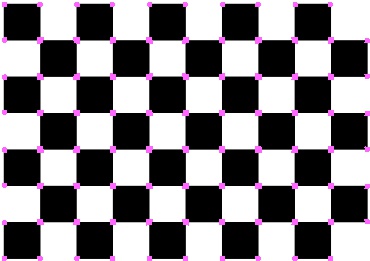
Corners are essentially regions of an image with considerable variations of intensity (assuming a monochrome image) in all directions. Take the picture below for instance, in every direction, there’s a different color. This is how the Harris corner detector finds corners: By taking the values of the pixels around a given pixel, it is able to determine whether or not the pixel is associated with a corner or not.
Applying the function
The code will be split up into 2 parts; a function I made for simplicity’s sake, followed by the Harris corner detector function.
import cv2
import numpy as np
window = 1
def imshow(img):
    global window
    name = "Window %d" %(window)
    window +=1
    cv2.imshow(name, img)
This first bit of the function really has nothing to do with the Harris Corner detector function itself. After doing a load of projects, you’ll realize how annoying it is to constantly specify a name for each of your windows with the cv2.imshow() function. This is especially a pain whilst debugging, so here’s a function called imshow() that simplifies this process, by taking an img as a parameter.
#insert image location in "loc"
loc = "C:\Users\user pc\Desktop\PPictures\chessboard.png"
img = cv2.imread(loc)
grey = cv2.cvtColor(img, cv2.COLOR_BGR2GRAY)
grey = np.float32(grey)

#use the harris corner function to locate corners
new = cv2.cornerHarris(grey, 5, 3, 0.04)

#Optimal value thersholding may vary from image to imag
img[new>0.01*new.max()]=[255,102,255]

#show the image
imshow(img)
cv2.imwrite('C:\Users\user pc\Desktop\PPictures\chessboardman.png',img)
cv2.waitKey(0)
cv2.destroyAllWindows()
OpenCV allows you to implement the corner detection algorithm in one neat, simple function, cv2.cornerHarris(img, blocksize, ksize, k). This function takes the following parameters:
img – Float 32 input image
blocksize – Determines the size of the neighborhood of surrounding pixels considered
ksize – Aperture parameter for Sobel (the x and y derivatives are found using the sobel function)
k – Harris detector free parameter
The above images are the results of the cv2.cornerHarris() function. On these still images, it works pretty well!
Since when did a super interesting blog become a bio lesson?
Sometimes you get inspired by the things you’re most horrible at. In my final year of school, I decided to face one of my biggest science-field nightmares, biology. However, if I’m doing bio, it’s on my terms. No memorizing for an exam or profusely exhibiting my medical adroitness through unnecessarily labyrinthine jargon. Also, I’m competing in a competition where I’m creating a neural network to detect pathogens in blood smears.
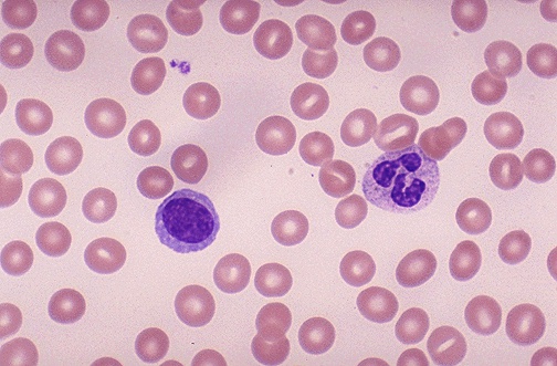
Introduction to blood smears
To put it concisely, a blood smear is essentially a microscopic image of your blood that contains a set of Red blood cells, white blood cells and other blood cell nonsense. It looks similar to this
These can reveal a lot about your present health. Blood morphology (viewing and understanding the composition of blood smear images) can point to the onset of leukemia, sickle cell, and also the presence of lymphocytes, monocytes, basophil’s etc. It generally requires a trained eye to detect all of this, but during the next few lessons, we’re going to see if we can make a computer segment the blood cells and understand them individually.
Prerequisites
A very solid foundation in OpenCV and Python; this exercise is just another big project you’ll be undertaking to hone your skills so you should ideally have a good understanding of the basic functions or if not, have the ability to look up and process the documentation.
Watershed? Why not contours?
For the sake of simplicity and to avoid too many gifs and animations, I’m just going to say it’s because you can learn an amazing new skill and learn how to implement it. However, if you’d like to see all the gifs and animations, check this brilliant page out. It’s where I learnt about watershed.
Morphology
In order to apply watershed, you’ll need to use morphological transformations and contrast enhancement in order to define boundaries and markers for the algorithm to take effect properly. Not doing these may lead to over-segmentation or under-segmentation.
#load your image, I called mine 'rbc'
img = cv2.imread('C:\Users\\user pc\Desktop\PPictures\\rbc.jpg')
#keep resizing your image so it appropriately identifies the RBC's
img = cv2.resize (img, (0,0), fx=5, fy=5)
#it's always easier if the image is copied for long pieces of code.
#we're copying it twice for reasons you'll see soon enough.
wol = img.copy()
gg=img.copy()
#convert to grayscale
img_gray = cv2.cvtColor(gg, cv2.COLOR_BGR2GRAY)
#enhance contrast (helps makes boundaries clearer)
clache = cv2.createCLAHE(clipLimit=2.0, tileGridSize=(8,8))
img_gray = clache.apply(img_gray)
#threshold the image and apply morphological transforms
_, img_bin = cv2.threshold(img_gray, 50, 255,
        cv2.THRESH_OTSU)
img_bin = cv2.morphologyEx(img_bin, cv2.MORPH_OPEN,
        numpy.ones((3, 3), dtype=int))
img_bin = cv2.morphologyEx(img_bin, cv2.MORPH_DILATE,
        numpy.ones((3, 3), dtype=int), iterations= 1)
#call the 'segment' function (discussed soon)
dt, result = segment(img, img_bin)
Apply watershed
Prior to applying watershed, a Euclidean distance transform is first implemented onto the frame. This evaluates the brightness of each pixel relative to it’s distance to a pixel with a ‘zero’ value. A zero value pixel is black, so EDT allows for a visualization of the how far any part of the image is from the background (which due to previous thresholding, should be black). You’ll notice that areas around the edge have a duller gray color, that slowly becomes a bright white color. We want to focus on the bright white color as our marker, because we’re sure it’s a part of the shape. The edges and duller colors are not 100%.
def segment(im1, img):
    #morphological transformations
    border = cv2.dilate(img, None, iterations=10)
    border = border - cv2.erode(border, None, iterations=1)
    #invert the image so black becomes white, and vice versa
    img = -img
    #applies distance transform and shows visualization
    dt = cv2.distanceTransform(img, 2, 3)
    dt = ((dt - dt.min()) / (dt.max() - dt.min()) * 255).astype(numpy.uint8)
    #reapply contrast to strengthen boundaries
    clache = cv2.createCLAHE(clipLimit=2.0, tileGridSize=(8,8))
    dt = clache.apply(dt)
    #rethreshold the image
    _, dt = cv2.threshold(dt, 40, 255, cv2.THRESH_BINARY)
    lbl, ncc = label(dt)
    lbl = lbl * (255/ncc)
    # Complete the markers
    lbl[border == 255] = 255

    lbl = lbl.astype(numpy.int32)
    #apply watershed
    cv2.watershed(im1, lbl)

    lbl[lbl == -1] = 0
    lbl = lbl.astype(numpy.uint8)
    #return the image as one list, and the labels as another.
    return dt, lbl
And there you have it! You can Segment most blood smear images in a few seconds! A major problem, however, is its lack of accuracy for different sized images of various resolutions and color textures. In order to improve the accuracy, I’ll soon be showing you how to do the same morphology, except with histogram equalization so you can more clearly define your boundaries.
Since you’re going to be working with an operating system, it’s best to know how exactly the system works so you can manipulate it in order to take full advantage of this virtually limitless tool.
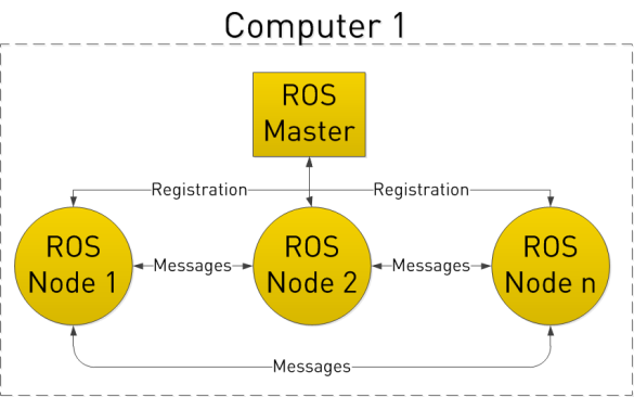
Nodes and Master
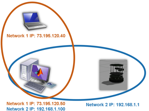
ROS is used primarily to establish a connection between modules, known as nodes. A node is just but some code that you can execute. Your ‘Hello world.py’ program is a node (albeit not a very useful one). ROS’s flexibility lies in the fact that these nodes can lie anywhere. You can have a node on your laptop, a node on a raspberry pi and another node on your desktop, and all of these nodes will work with each other to make your robot function. The advantage of this distribution is to organize system control. For a robot that processes and image, finds a face and then drives towards said face, you can have a node for receiving camera images and processing them and another node for controlling the steering of the robot in response.
Nodes
Nodes perform and action; they’re actually just software modules but can communicate with other nodes and register with the master (we’ll get to that). These nodes can be created in a number of ways. You can type up a command in a terminal window to create a node or you can create them using Python or C++ as a script.
Nodes Publish and Subscribe
In ROS, a series of task
s can be split into a series of simpler tasks (both, simplicity in execution and simplicity of code can be achieved) . For a wheeled robot the tasks can include the perception of the environment using a camera or laser scanner, map making, planning a route, monitoring the battery level of the robot’s battery, and controlling the motors driving the wheels of the robot.
Some nodes provide information to others. The feedback from the camera is an example. This node is said to publish information to other nodes.
A node that receives the camera image is subscribed to the other node. As an example, The wheels could be subscribed to a camera, which is publishing.
In some cases, a node can both publish and subscribe to one or more topics. You’ll see more of those as you progress.
ROS Master
If nodes were like railway stations in a complicated subway, ROS master is like the map. ROS master provides naming and registration services to individual nodes and allows them to locate with each other. It does so primarily using the TCP/IP, called TCPROS. In short, this enables communication over the Internet.
Enough of the boring theory, in the next lesson, we’ll get more hands on. For more information on how to list nodes and other handy tips, go to this website.
A catkin workspace is where you’ll be able to modify existing or create new catkin packages. The catkin structure simplifies the build and install process for your ROS packages.
Create it
Naming our folder catkin_ws, Just type in the following into terminal to create the workspace.
 mkdir –p ~/catkin_ws/src
 cd ~/catkin_ws/src$ catkin_init_workspace
Next, build it by following up with:
 cd ~/catkin_ws/
 catkin_make
Overaly the workspace atop your ROS environment by sourcing setup.bash
Here you’ll be installing ROS indigo (which is just a distribution of ROS, like Ubuntu is a distribution of Linux). I recommend ROS indigo because it is the most stable version to date and will have support until 2019. It also supports the latest version of Ubuntu.
Setup your sources.list
Setup your computer to accept software from packages.ros.org. ROS Indigo ONLY supports Saucy (13.10) and Trusty (14.04) for Debian packages.
The ROS system may depend on software packages that are not loaded initially. These software packages external to ROS are provided by the operating system. The ROS environment command rosdep is used to download and install these external packages. It’s kind of like the way you use sudo apt-get install, except since ROS is a different operating system, you use this.
Type the following command:
sudo rosdep init
rosdep update
Setup ROS environment
source /opt/ros/indigo/setup.bash
Sometimes it’s easier if the variables are automatically added to your sessions every time a new shell is launched. Do so by typing the following command into terminal.
Arduino. OpenCV. Kinect. AR Drone. CrazyFlie. Turtlebot. SLAM. 3D Mapping.
Some of those words may be familiar to you, some of them may not. There was a time when Robotics for us revolved around the Lego NXT and EV3 sets. After a few years, we got fed-up of only using 3 motors and 4 sensors and paying a ton for the extra stuff. That’s when we began working with the Arduino, making little ultrasonic sensor bots and enjoying a 16 servo robotic spider. If you’re done impressing people with that stuff (or just want to skip it altogether), read on:
Well there’s a step ahead of that, which allows you to use the tools of a Real Roboticist and expand any horizons in robotics you though ever limited you.
Dive into the world of the ROBOTIC OPERATING SYSTEM (ROS)
ROS is much like an operating system, but uses Linux to run. If you’re here, then you probably know the world of things ROS can do for advancing your robotics knowledge.
ROS can help you:
Create vivid and accurate 3D reconstructions of your environment. The maxed-out team did something like this for their project.
Completely automate drones and engage in localization in indoor environments like the Parrot AR drone, the Parrot Bebop drone. Upenn students used ROS to achieve this:
Create amazing simulations of robots and allow them to interact with the environment, creating the perfect testing tool before actually creating your robot.
Integrate it with the libraries you know, like OpenCV, numpy and scipy, even the Arduino IDE to create some amazing robots that could truly work under a range of situations.
Although it may be cliche to say this, especially now, the possibilities are absolutely endless.
There’s also a wealth of documentation online , so you can be sure that you’ll never ever run into a problem and get stuck for too long.
That being said, there are some prerequisites before you continue. You need to be good at Python, and have at least some remote understanding of how the Terminal works on Linux.
All that being said, continue on to the next lesson to learn how to install ROS Indigo on your Ubuntu LTS 14.04 .
Brushless motors come in handy when your project requires high RPM and low maintenance. A fantastic video by 000Plasma000 explains the properties of brushless motors very concisely.
UPDATE: WordPress is changing some of my code blocks to ‘amp’ and I haven’t yet found a way to fix this. For further guidance (although it would be a good exercise to infer), head over to my github repository.
Lithium Polymer (LiPo) Battery. These are essentially the same batteries used by FPV drones or planes or RC cars.
Power Distribution Board (optional, if you want to connect more than one brushless motor to the Arduino)
Software:
Arduino IDE
Making the connections
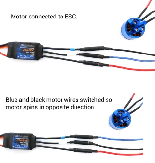
For all intents and purposes, you will be treating an ESC+Brushless motor combo as if it were a servo. You’ll see this application in action soon, but for now, follow the diagram and instructions to connect the Motor to the ESC and the ESC to the Arduino.
The ground and power wires of the Motor can be interchanged with each other in plugging into the ground and power slots on the ESC. It doesn’t matter where these wires go, as long as they stay on the outside, switching them will just switch the direction. The signal wire must connect with the middle wire on the ESC as this transmits the signal. Different motors and ESC’s have different arrangements for this, so it is up to you to figure out which wire carries the signal on both the ESC and Motor so you can mess about with the other two any way you like.
There will be 3 thin wires from the ESC. These will be differently colored, but one of these will be for powerinput, one for the Signal and one that goes to ground. You must research the color coding of your wires and then accordingly plug the signal wire into PWM port 9 and the Ground wire to GND. DO NOT PLUG THE POWER INPUT WIRE INTO THE ARDUINO, you may fry your computer’s USB port along with the Arduino.
Arduino Code
#include <Servo.h>

int value = 0; // set values you need to zero

Servo firstESC, secondESC; //Create as many as Servo objects as you want. You can control 2 or more Servos at the same time

void setup() {

  firstESC.attach(9);    // attached to pin 9 I just do this with 1 Servo
  Serial.begin(9600);    // start serial at 9600 baud (can change this)

}

void loop() {

//First connect your ESC WITHOUT Arming. Then Open Serial and follow Instructions

  firstESC.write(value);

  if(Serial.available())
    value = Serial.parseInt();    // Parse an Integer from Serial

}
As is evident, we’re treating the ESC as if it were a servo object. You can add more servo objects if you like, just connect them to a breadboard and to more PWM’s. This code will allow you to send a value through the serial monitor on your Arduino IDE, and control the speed of your ESC’s accordingly
My Setup
Start by connecting the ESC to the battery. You should hear a little beep. Then, connect the USB to the Arduino and load the program. You should hear another beep. Nevertheless, this all depends on what kind of ESC you have. Mine had black, white and red , White was for the signal, so that went to PWM port 9. Black was for ground so that went to ground.
Brushless Motor’s in Action
The following video show’s my brushless motors in action. I vary the serial input from 10 to around 150, and as expected, higher values result in higher RPM.


