The right way to connect an HC-05 Bluetooth module to an Arduino (Running Linux Ubuntu)

The HC-05 Bluetooth module is extremely useful for wireless communication and will last long if you know how to use it correctly.

UPDATE: WordPress is changing some of my code blocks to ‘amp’ and I haven’t yet found a way to fix this. For further guidance (although it would be a good exercise to infer), head over to my github repository.

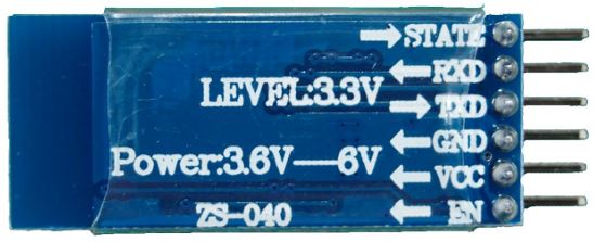
The first mistake people make when rushing to get the HC-05 module is when they connect the TX from the Arduino directly to the RX in the Hc-05. However, the TX on the Arduino transmits a 5 volt (5v) signal, whereas the RX  on the Hc-05 accepts only upto 3.3 volts (3v). Here’s a picture for proof:

Notice how the RX (same as RXD) has Level 3.3V. Any more and you could risk blowing up your Bluetooth module!

Breadboarding

So start off by getting it wired on your breadboard the following way. The resistors used in this positioning allow 5v to drop to 3.3v , allowing you to communicate with your bluetooth module safely.

At this point, you should only care about those 4 pins on the Hc-05. Don’t worry about the rest. (State and EN)

For the resistor setup, understand the following: The easiest way to go about this is by picking 3 resistors of the same type. I would suggest something in the 1K – 10K range. To understand more about how exactly this voltage divider works, visit this website .

Install Blueman Bluetooth Manager (for Ubuntu 14.04)

This is a useful bluetooth manager and will allow the HC-05 to connect to a comm port on your laptop with ease. Just open terminal and type in the following two lines of code:

sudo apt-get update
sudo apt-get install blueman

 

Install CuteCom (for Ubuntu 14.04 )

If you’re running Ubuntu, you should install Cutecom. It will allow you to read from your connected comm port. Just type in the following two lines of code in the Terminal:

sudo apt-get update
sudo apt-get install cutecom

Arduino Code

This is the .ino code you should compile. You can either copy paste this into the Arduino IDE or download the .ino file below itself.

int counter =0;
char INBYTE;
void setup() {
  pinMode(13, OUTPUT);
  Serial.begin(9600);
  delay(50);
}

void loop() {
  counter++;
  Serial.println("Press 1 to turn on LED and 0 to turn off ");
  while (true){
    if (Serial.available()){
      break;
    }
  }
  INBYTE = Serial.read();
  if (INBYTE == '0'){
    digitalWrite(13, LOW);

  }
  if (INBYTE == '1'){
    digitalWrite(13, HIGH);
  }
  Serial.println(counter);
  delay(50); // wait half a sec
}

Testing the Module

I will cover troubleshooting in another tutorial, but at this point, following these instructions should get everything working fine.

1.  Remove the RX and TX connection from the arduino. This is temporary. Do not remove the wire entirely, just disconnect the end’s that are connected to the Arduino’s RX and TX ports.
2. Download the following tester code or copy paste it from above: BLUETOOTH_TEST.ino
3. Compile this code onto the Arduino.
4. Disconnect the USB from the Arduino (very important).
5. Attach a 9V battery with a barrel jack to the Arduino.
6. Open Bluetooth Manager and walk yourself through setting up the device.
   You should see something like this:

This slideshow requires JavaScript.

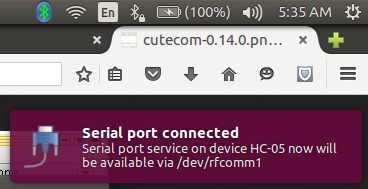
7.Once you’re done setting up, this notification should pop on the screen. Take note of the rfcomm number. These will be of the form /dev/rfcomm0 or /dev/rfcomm1 etc.

8.Open a Terminal

      9.Type in cutecom

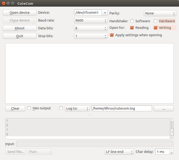
1. Where it says Device: , change the name to whichever rfcomm port your HC-05 is connected to.
2. Set the Baud rate to 9600
3. Click Open Device 
4. You should see the text box below open up.
5. Press 1 to turn on LED and 0 to Turn it off.

Torch/Flashlight blob tracker using Python and OpenCV

Tracking the blob of light from a flashlight can be useful. It certainly was for my Google Science fair project, and it may also be useful for any projects of your own. So without further ado, here’s the flashlight blob tracker.

Prerequisites

You should be able to understand the code in my previous post and should also have a strong foundation in python.

Create new thresholded frame

So far, we’ve been using the cv2.cvtColor() function simply in order to convert from an BGR colorspace to an HSV colorspace. But HSV colorspaces are only useful for thresholding specific colors or color ranges. This won’t work for thresholding a certain brightness. We’ll need a different colorspace for this.

#import libs
import cv2
import numpy as np
import time

#begin streaming
cap = cv2.VideoCapture(0)
while True:
    _, frame = cap.read()

    #convert frame to monochrome and blur
    gray = cv2.cvtColor(frame, cv2.COLOR_BGR2GRAY)
    blur = cv2.GaussianBlur(gray, (9,9), 0)

    #use function to identify threshold intensities and locations
    (minVal, maxVal, minLoc, maxLoc) = cv2.minMaxLoc(blur)

    #threshold the blurred frame accordingly
    hi, threshold = cv2.threshold(blur, maxVal-20, 230, cv2.THRESH_BINARY)
    thr = threshold.copy()

    #resize frame for ease
    cv2.resize(thr, (300,300))

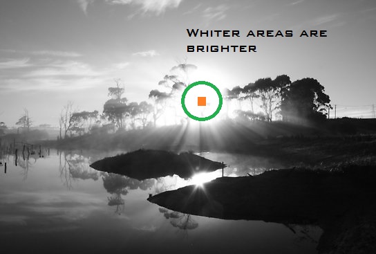
cv2.cvtColor(frame, cv2.COLOR_BGR2GRAY). The unfamiliar parameter should be self explanatory, cv2.COLOR_BGR2GRAY, converts a frame from the BGR colorspace to the ‘gray’ or ‘monochrome’ colorspace. The reason this is done is intuitive. In a black and white image, the brightest area generally also appears to be the most white area in the picture. (The sun is the whitest area in this picture, and we know that it is also the brightest area in the picture).

cv2.minmaxloc() is also fairly self-explanatory. It searches the frame and returns the brightest pixel, the darkest pixel, and their respective positions. These values are then used as thresholds in threshold  frame. Our thresholded frame is called thr and threshold.

Identify light blob in thresholded frame

    #find contours in thresholded frame
    edged = cv2.Canny(threshold, 50, 150)
    lightcontours, hierarchy = cv2.findContours(edged, cv2.RETR_TREE, cv2.CHAIN_APPROX_SIMPLE)

    #attempts finding the circle created by the torch illumination on the wall
    circles = cv2.HoughCircles(threshold, cv2.cv.CV_HOUGH_GRADIENT, 1.0, 20,
                               param1=10,
                               param2= 15,
                               minRadius=20,
                               maxRadius=100,)

We use the cv2.HoughCircles function simply because one can intuitively confirm that a blob of light from a flashlight on a wall resembles a circular figure. NOTE: YOU MUST MESS AROUND WITH THE PARAMETERS ON THE HOUGH CIRCLES FUNCTION UNTIL  FALSE DETECTIONS ARE MINIMIZED

Track the light blob

All we have left is to make sure the blob detected matches the type we’re tracking for and then draw a marker around this light blob.

    #check if the list of contours is greater than 0 and if any circles are detected
    if len(lightcontours)>0 and circles is not None:
        #Find the Maxmimum Contour, this is assumed to be the light beam
        maxcontour = max(lightcontours, key=cv2.contourArea)
#avoids random spots of brightness by making sure the contour is reasonably sized
        if cv2.contourArea(maxcontour) > 2000:
            (x, final_y), radius = cv2.minEnclosingCircle(maxcontour)
            cv2.circle(frame, (int(x), int(final_y)), int(radius), (0, 255, 0), 4)
            cv2.rectangle(frame, (int(x) - 5, int(final_y) - 5), (int(x) + 5, int(final_y) + 5), (0, 128, 255), -1)
#display frames and exit
    cv2.imshow('light', thr)
    cv2.imshow('frame', frame)
    cv2.waitKey(4)
    key = cv2.waitKey(5) & 0xFF
    if key == ord('q'):
        break
cap.release()
cv2.destroyAllWindows()

Line 2 is to avoid an error that will appear if no circular light blobs are detected. If none are detected, the code just passes this iteration.

Line 4 assumes the light blob is the largest sized circular blob in the entire frame, meaning the maxcontour would be the blob itself.

Lines 6 is to make sure any tiny blobs or random bright pixels due to glare or other environmental interferences are not detected. The area must be over a certain value to be considered legit.

Lines 7-18  Just draw the trackers and display the frame.

Live camera-based angle calculator using python and OpenCV

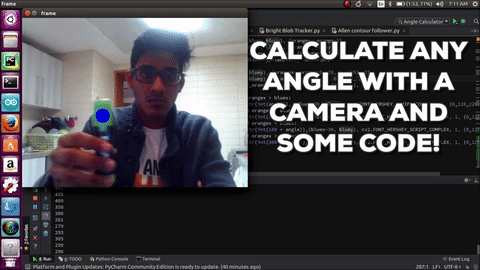
After building a portion of your foundation, it’s best to continue learning by building something that’s not only useful, but also looks insanely impressive. So here you have it, a basic angle calculator.

UPDATE: WordPress is changing some of my code blocks to ‘amp’ and I haven’t yet found a way to fix this. For further guidance (although it would be a good exercise to infer), head over to my github repository.

LINK TO GITHUB GIST WITH ANGLECALC: https://gist.github.com/botforge/c88b842cafaa077a91048d51c2db0bdf

Prerequisites

This tutorial assumes you have some degree of proficiency with Python and can reasonably understand the OpenCV code here.

Determine HSV Range (again)

Before you continue writing the code you’ll need to use this HSV Trackbar to determine the Hue Low/High, Saturation Low/High and Value Low/High for the object you want to track. Mess around with the trackbars until you can only see the color of the object you are looking for. Repeat this process twice, for 2 differently colored objects. Note these values down, you will need them for later.

Filter for HSV Colors

Creating functions makes life a billion times easier, and allows you to organize your code much more effectively. I wrote the code initially with the functions findorange and findblue , although I eventually ended up using green and orange.

#import libs
import cv2
import numpy as np
import math

#uses distance formula to calculate distance
def distance((x1, y1), (x2,y2)):
    dist = math.sqrt((math.fabs(x2-x1))**2+((math.fabs(y2-y1)))**2)
    return dist

#filters for blue color and returns blue color position.
def findblue(frame):
    maxcontour = None
    blue = cv2.cvtColor(frame, cv2.COLOR_BGR2HSV)
    bluelow = np.array([55, 74, 0])#replace with your HSV Values
    bluehi = np.array([74, 227, 255])#replace with your HSV Values
    mask = cv2.inRange(blue, bluelow, bluehi)
    res = cv2.bitwise_and(frame, frame, mask=mask)

#filters for orange color and returns orange color position.
def findorange(frame):
    maxcontour = None
    orange = cv2.cvtColor(frame, cv2.COLOR_BGR2HSV)
    orangelow =  np.array([0, 142, 107])#replace with your HSV Values
    orangehi = np.array([39, 255, 255])#replace with your HSV Values
    mask = cv2.inRange(orange, orangelow, orangehi)
    res = cv2.bitwise_and(frame, frame, mask=mask)

Just remember to change the bluelow and bluehi and orangelow and orangehi array’s elements to those that suit your color choice. All of the functions used should be familiar from my tutorial on ‘Object Tracking and Following with OpenCV Python‘; read that if you don’t get some of it. What we’ve essentially done is sent the initial frame as a parameter to each of these functions, where they then convert to HSV and threshold for the color.

Return object positions

Next, you want to continue building on findblue() and findorange() by allowing them to return the coordinates of your objects.

def findblue(frame):
    blue = cv2.cvtColor(frame, cv2.COLOR_BGR2HSV)
    bluelow = np.array([55, 74, 0])#replace with your HSV Values
    bluehi = np.array([74, 227, 255])#replace with your HSV Values
    mask = cv2.inRange(blue, bluelow, bluehi)
    res = cv2.bitwise_and(frame, frame, mask=mask)
    cnts, hir = cv2.findContours(mask, cv2.RETR_TREE, cv2.CHAIN_APPROX_SIMPLE)
    if len(cnts) >0:
        maxcontour = max(cnts, key = cv2.contourArea)

        #All this stuff about moments and M['m10'] etc.. are just to return center coordinates
        M = cv2.moments(maxcontour)
        if M['m00'] > 0 and cv2.contourArea(maxcontour)>2000:
            cx = int(M['m10'] / M['m00'])
            cy = int(M['m01'] / M['m00'])
            return (cx, cy), True
        else:
            #(700,700), arbitrary random values that will conveniently not be displayed on screen
            return (700,700), False
    else:
        return (700,700), False

#filters for orange color and returns orange color position.
def findorange(frame):
    orange = cv2.cvtColor(frame, cv2.COLOR_BGR2HSV)
    orangelow =  np.array([0, 142, 107])#replace with your HSV Values
    orangehi = np.array([39, 255, 255])#replace with your HSV Values
    mask = cv2.inRange(orange, orangelow, orangehi)
    res = cv2.bitwise_and(frame, frame, mask=mask)
    cnts, hir = cv2.findContours(mask, cv2.RETR_TREE, cv2.CHAIN_APPROX_SIMPLE)
    if len(cnts) >0:
        maxcontour = max(cnts, key = cv2.contourArea)
        M = cv2.moments(maxcontour)
        if M['m00'] > 0 and cv2.contourArea(maxcontour)>2000:
            cx = int(M['m10'] / M['m00'])
            cy = int(M['m01'] / M['m00'])
            return (cx, cy), True
        else:
            return (700,700), False
    else:
        return (700,700), False

The cv2.Moments function and the cx and cy variable declarations are best explained in OpenCV’s introduction to contours. But simply put, lines n – n just return the coordinates of the center of the contour.

The reason we have the blogic boolean variable is just to validate that the object is present on screen. If the object isn’t present, this variable will be set to False, and the coordinates will be (700,700). I chose this set of points arbitrarily, as these, even when plotted, couldn’t be seen on my 300 x 400 window.

Distance Function

We’ll be using trigonometry to calculate the angle, so for this you’ll need to create a function that measures the distance between both points. For this, we use the standard distance equation  you should’ve learnt in high school.

#uses distance formula to calculate distance
def distance((x1, y1), (x2,y2)):
    dist = math.sqrt((math.fabs(x2-x1))**2+((math.fabs(y2-y1)))**2)
    return dist

 

Main Loop

#capture video
cap = cv2.VideoCapture(0)

while(1):
    _, frame = cap.read()
#if you're sending the whole frame as a parameter,easier to debug if you send a copy
    fra = frame.copy() 

     #get coordinates of each object
    (bluex, bluey), blogic = findblue(fra)
    (orangex, orangey), ologic = findorange(fra)
    #draw two circles around the objects (you can change the numbers as you like)
    cv2.circle(frame, (bluex, bluey), 20, (255, 0, 0), -1)
    cv2.circle(frame, (orangex, orangey), 20, (0, 128, 255), -1)

Our foundation is set. We’ve made a program that tracks the position of 2 different colored objects on screen, next, we need to apply trig to calculate the angle and display the entire setup in the most grandiose manner possible.

    if blogic and ologic:
        #quantifies the hypotenuse of the triangle
        hypotenuse =  distance((bluex,bluey), (orangex, orangey))
        #quantifies the horizontal of the triangle
        horizontal = distance((bluex, bluey), (orangex, bluey))
        #makes the third-line of the triangle
        thirdline = distance((orangex, orangey), (orangex, bluey))
        #calculates the angle using trigonometry
        angle = np.arcsin((thirdline/hypotenuse))* 180/math.pi

        #draws all 3 lines
        cv2.line(frame, (bluex, bluey), (orangex, orangey), (0, 0, 255), 2)
        cv2.line(frame, (bluex, bluey), (orangex, bluey), (0, 0, 255), 2)
        cv2.line(frame, (orangex,orangey), (orangex, bluey), (0,0,255), 2)

Our code is officially complete…sort of. If you run it, it’ll look great and work great but you’ll notice that it won’t detect any angle over 90 degrees. If you’re familiar with trig, you’ll know why, but to evade this situation and allow it to calculate angles until 180 degrees, we need a few more lines of code.

     #Allows for calculation until 180 degrees instead of 90
if orangey < bluey and orangex > bluex:
    cv2.putText(frame, str(int(angle)), (bluex-30, bluey), cv2.FONT_HERSHEY_SCRIPT_COMPLEX, 1, (0,128,220), 2)
elif orangey < bluey and orangex < bluex:
    cv2.putText(frame, str(int(180 - angle)),(bluex-30, bluey), cv2.FONT_HERSHEY_SCRIPT_COMPLEX, 1, (0,128,220), 2)
elif orangey > bluey and orangex < bluex:
    cv2.putText(frame, str(int(180 + angle)),(bluex-30, bluey), cv2.FONT_HERSHEY_SCRIPT_COMPLEX, 1, (0,128,220), 2)
elif orangey > bluey and orangex > bluex:
    cv2.putText(frame, str(int(360 - angle)),(bluex-30, bluey), cv2.FONT_HERSHEY_SCRIPT_COMPLEX, 1, (0,128, 229), 2)
if k == ord('q'): break

And that’s it! If the object tracker didn’t impress already, now you have a live angle calculator using just your camera.

Object Tracking and Following with OpenCV Python

Object tracking and the concepts learnt from developing an object tracking algorithm are necessary for computer vision implementation in robotics. By the end of this tutorial, you will have learnt to accurately track an object across the screen.

UPDATE: WordPress is changing some of my code blocks to ‘amp’ and I haven’t yet found a way to fix this. For further guidance (although it would be a good exercise to infer), head over to my github repository.

Prerequisites

This tutorial assumes you have some degree of proficiency with Python and can reasonably understand the OpenCV code here.

Determine HSV Range

Before you continue writing the code you’ll need to use this HSV Trackbar to determine the Hue Low/High, Saturation Low/High and Value Low/High for the object you want to track. Mess around with the trackbars until you can only see the color of the object you are looking for. Note these values down, you will need them for later.

Filter for HSV Color

#import necessary libraries
import cv2
import numpy as np
import time
#initialize the video stream
cap = cv2.VideoCapture(0)

#make two arrays, one for the points, and another for the timings
points = []
timer = []
while True:
    #start the timing
    startime = time.time()

    #append the start time to the array named 'timer'
    timer.append(g)

    #you only want to use the start time, so delete any other elements in the array
    del timer[1:]
    _, frame = cap.read()

    #resize and blur the frame (improves performance)
    sized = cv2.resize(frame, (600, 600))
    frame = cv2.GaussianBlur(sized, (7, 7), 0)

    #convert the frame to HSV and mask it
    hsv = cv2.cvtColor(frame, cv2.COLOR_BGR2HSV)
#fill in the values you obtained previously over here
    hlow = 17
    slow = 150
    vlow = 24
    hhigh = 78
    shigh = 255
    vhigh = 255
    HSVLOW  = np.array([hlow, slow, vlow])
    HSVHIGH = np.array([hhigh, shigh, vhigh])
    mask = cv2.inRange(hsv,HSVLOW, HSVHIGH)
    res = cv2.bitwise_and(frame,frame, mask =mask)

All of this stuff should be pretty straightforward after a few read-through’s. The only new function here is cv2.resize() and that itself is quite self explanatory (it resizes the frame). At this point, we have our new, ‘thresholded’ frame.

As a word of advice, make sure there isn’t a huge concentration of the color you’re looking for on the screen. For this basic object tracker, we’re only relying on color so if you have a lot of the color you want to track in the background, your best bet is to find a different colored object.

Find Maximum Contour

A lot of the time, you can simply visualize the algorithm necessary for solving most computer vision problem for robots if you understand what contours are. Since it is such a powerful tool, I suggest you build your foundation at this link (do the exercises, don’t just read), and come back when you kind of understand what contours are.

Once your done, try understanding this code.

    #create an edged frame of the thresholded frame
    edged = cv2.Canny(res, 50, 150)

    #find contours in the edged frame and append to the 'cnts' array
    cnts = cv2.findContours(edged, cv2.RETR_TREE, cv2.CHAIN_APPROX_SIMPLE)[0]

    # if contours are present
    if len(cnts)> 0:

        #find the largest contour according to their enclosed area
        c = max(cnts, key=cv2.contourArea)

        #get the center and radius values of the circle enclosing the contour
        (x, y), radius = cv2.minEnclosingCircle(c)

 

We started with the cv2.Canny()  function (documentation) with a min and max  threshold. Ignore the technicalities of the numbers, that essentially finds all of the edges in the frame.

Since cv2.findContours() returns a list, we need to find the largest contour (which we assume is our object) in this list. We use the max(cnts, key=cv2.contourArea). Thus, this function finds the area of all of the contours in the list, and then returns it’s maximum.

Following that we use the cv2.minEnclosingCircle(c) function to find the (x,y) coordinates of the center of the circle, and it’s radius.

At this point, we have tracked our object in the frame. All that’s left is to draw the circle and the trailing line. 

        centercircle = (int(x), int(y))
        radius = int(radius)
        cv2.circle(sized, centercircle, radius, (255, 30,255), 2) #this circle is the object
        cv2.circle(sized, centercircle, 5, (0, 0, 255), -1) #this circle is the moving red dot
        points.append(centercircle) #append this dot to the 'points' list
        if points is not None:
            for centers in points:
                cv2.circle(sized, centers, 5, (0, 0, 255), -1) #make a dot for each of the points

    #show all the frames and cleanup
    cv2.imshow('frame', sized)
    cv2.imshow('mask', res)
    k = cv2.waitKey(5) & 0xFF
    g = time.time()
    timer.append(g)

    #if 10 seconds have passed, erase all the points
    delta_t = timer[1] - timer[0]
    if delta_t >= 10:
        del timer[:]
        del points[:]
    if k == 27:
        break

Lines 1-9 essentially draw the circle around the object, and draw another small red circle at it’s center. This dot constitutes a point in the trail.  This point is then appended to the existing array ‘points’.

The for loop that follows cycles through each of the centers’ (x,y) coordinates (from the ‘points’ array) and draws another red dot in each position, effectively creating the trail.

Finally, another value is appended to the timer array. Delta_t computes the difference between the start and final times. If this value is greater than 10, all points are erased and a new trail is begun.

 

Color trackbar/slider using OpenCV Python

By the end of this post, you’ll have made a pretty basic HSV color trackbar/slider that filters out a range of colors, leaving you with the range of colors that you want to identify. HSV stands for ‘Hue, Saturation, Value’. It is composed of 3 separate values that determine the range of colors that you’d want to find.

If you just want the code, follow this link to my github

https://github.com/botforge/ColorTrackbar/blob/master/HSV%20Trackbar.py

Prerequisites

This tutorial assumes you have some degree of proficiency with Python and have dabbled around with OpenCV. If you haven’t touched OpenCV ever, this tutorial still has links to whatever you may need to know to complete writing this code.

1. Creating Trackbars

OpenCV has a pretty good tutorial on creating and reading multiple trackbars, but it digresses from the application we intend to use it for. Carefully reading the following section should suffice.

Don’t worry if you don’t get some of it, I’ll explain the important functions soon.

#import the necessary packages
import cv2
import numpy as np
#'optional' argument is required for trackbar creation parameters
def nothing:
pass

#Capture video from the stream
cap = cv2.VideoCapture(0)
cv2.namedWindow('Colorbars') //Create a window named 'Colorbars'

#assign strings for ease of coding
hh='Hue High'
hl='Hue Low'
sh='Saturation High'
sl='Saturation Low'
vh='Value High'
vl='Value Low'
wnd = 'Colorbars'
#Begin Creating trackbars for each
cv2.createTrackbar(hl, wnd,0,179,nothing)
cv2.createTrackbar(hh, wnd,0,179,nothing)
cv2.createTrackbar(sl, wnd',0,255,nothing)
cv2.createTrackbar(sh, wnd,0,255,nothing)
cv2.createTrackbar(vl, wnd,0,255,nothing)
cv2.createTrackbar(vh, wnd',0,255,nothing)

You may be wondering what the parameters of the cv2.createTrackbar() function are. The OpenCV documentation is the best place for a comprehensive explanation, but I’ll give you one more specific to the problem we’re solving.

So the parameters are as follows:

cv2.createTrackbar(trackbarname, windowname, minimum, maximum, argument)

We assigned our trackbar names in lines 13-18 and our window name in line 19. The minimum position of the trackbar for all instances is 0. In simpler terms, when you slide the slider, it won’t go below a value of 0 as no HSV values are negative. The maximum  position varies. For the Hue values it goes from 0-180, and for Saturation and Val, it goes from 0-255.

There’s no need to concern yourself with why those numbers were chosen, but if your interested, there are a bunch of books by O’Reilly on safaribooksonline.com to learn about the mathematics behind computer vision.

2. Reading and processing Trackbars

Here’s where the real stuff comes in. As usual, don’t fret if you don’t get the code, but try reading and understanding as much as you can.

#begin our 'infinite' while loop
while(1):
    #read the streamed frames (we previously named this cap)
    _,frame=cap.read()

    #it is common to apply a blur to the frame
    frame=cv2.GaussianBlur(frame,(5,5),0)

    #convert from a BGR stream to an HSV stream
    hsv=cv2.cvtColor(frame, cv2.COLOR_BGR2HSV)

All we did here was read the stream we previously assigned as cap.

Reading  the frame using the x.read() function returns a tuple. You can ignore the first value for now, and call the second value frame. This frame variable is actually an array of values. Each element of this array contains BGR (Blue, Green, Red) values. Concretely, each element is a pixel.

We also introduced a Gaussian Blur. This is commonly applied in order to reduce single pixel anomalies while searching the array. Read more about the Gaussian blur function here, but for the sake of simplicity, just remember that the first parameter is the array of pixels you receive from cap.read(), and the other numbers can generally remain untouched. 

The conversion between BGR to HSV is analogous to the conversion between mp3 and wav for your music files. You’re essentially converting the data in the frame so it becomes readable in a different way. That’s what the cv2.cvtColor() function does. You then name your new array ‘hsv‘

    #read trackbar positions for each trackbar
    hul=cv2.getTrackbarPos(hl, wnd)
    huh=cv2.getTrackbarPos(hh, wnd)
    sal=cv2.getTrackbarPos(sl, wnd)
    sah=cv2.getTrackbarPos(sh, wnd)
    val=cv2.getTrackbarPos(vl, wnd)
    vah=cv2.getTrackbarPos(vh, wnd)

    #make array for final values
    HSVLOW=np.array([hul,sal,val])
    HSVHIGH=np.array([huh,sah,vah])

#create a mask for that range
mask = cv2.inRange(hsv,HSVLOW, HSVHIGH)

The stuff above is pretty self explanatory. You read the trackbars with cv2.getTrackbarPos() and assign them to variables (you can name them anything).

In lines 10-11, your final frame shouldn’t show the whole frame, it should only show the range specified by your trackbar. To do that, you have to make a numpy array with the lower HSV values, and one with your higher HSV values. You then have to create a mask to apply this range to the frame. That’s what cv2.inRange()  does.

    res = cv2.bitwise_and(frame,frame, mask =mask)

    cv2.imshow(wnd, res)
    k = cv2.waitKey(5) && 0xFF
    if k == ord('q'):
        break

cv2.destroyAllWindows()

The cv2.bitwise_and function allows you to display your mask (the HSV image with the filtered range) back onto your initial frame. cv2.imshow() takes 2 parameters, namely, window name and image array. We’ll keep our initial window name, and we’ll choose to display the res array, as that contains the filtered array displayed on the initial frame.

Lines 4-6 just allows you to quit the whole process by pressing ‘q’.

That’s about it. Now dabble around with the trackbars to find your desired color range. Next, Learn how to track a filtered object across the screen.